MATH USED IN BLACKJACK
This section describes some of the mathematical and statistical ideas that are part of the game.
Expected Value
Whenever someone makes a wager, he is evaluating the risk of losing against the reward of winning. This risk-reward evaluation is quantified by expected value (EV), which weighs the bet by the probability-of-losing and the payoff by the probability-of-winning. The difference between the two is the expected value.
EV = (Payoff x Probability of Winning) - (Bet x Probability of Losing)
A positive and negative EV tells the gambler that the bet is good or bad. Investors use a similar technique to evaluate their investments.
Let’s try it with a coin toss, a $1 bet, and a one-for-one (1:1) payoff:
Payoff = $1
Probability of Winning = 50% (one out of two possible coin faces)
Bet = $1
Probability of Losing = 50% (one out of two possible coin faces)
Using the EV formula, we get an expected value $0:
Expected Value (coin toss) = ($1 x 50%) - ($1 x 50%) = $.50 - $.50 = $0
This means that the bettor should expect to win $0 on every coin-toss bet, which he will on average if he plays long enough. Based on this, there’s nothing to gain or lose on this bet.
However, something here doesn’t make sense as a single coin-toss is never going to return $0 as the EV analysis predicts; the payoff is always going to be minus $1 or plus $1 as the bettor is always going to win or lose his bet of $1. This is because expected value is subject to the Law of Large Numbers — the more samples (coin tosses in our example), the closer the average will come to the expected value. In other words, EV is the anticipated outcome of the average of many samples.
Let’s try another example, but this time let’s lower the payoff on the coin toss to $.90 for each $1 bet.
Payoff = $.90
Probability of Winning = 0.5 or 50%
Bet = $1
Probability of Losing = 0.5 or 50%
Expected Value (coin toss) = ($.90 x .5)-($1 x .5)=$.45-$.50= -$.05
Here the expectation is that on average the bettor will lose $.05 on every one-dollar bet.
Let’s try another example … a spinning wheel with 100 numbers and a $95 payoff on a $1 bet.
Payoff = $95
Probability of Winning = 0.01 (1 number out of 100)
Bet = $1
Probability of Losing = 0.99 (99 numbers out of 100)
Expected Value (spin wheel) = ($95 x .01)-($1 x .99)=$.95-$.99= -$.04
The expectation here is that the bettor will lose $.04 on every one-dollar bet (or $4 on 100 one-dollar bets). This spinning-wheel bet, however, is different from the other example. Here, the bettor is putting $1 at risk and he has the chance of winning $95. Not a bad deal despite the negative EV. This illustrates a typical lottery-like bet where it’s the generous payoff that motivates the bettor rather than the EV. Keno, for example, has an EV of minus $.40 for every $1 bet (or $40 for 100 one-dollar bets), but its payoff often is in the millions.
Expected Value is the average amount a bettor should expect to win or lose on a bet.
House Edge
The EV for a casino is called the house edge.
In the spinning wheel example, for instance, the player’s EV was minus $0.04 on every one-dollar bet. If we turn this around, the EV for the house is a positive $0.04 on every one-dollar bet or 4%. In other words, the casino has a 4% edge over the player. So, if a player makes 1,000,000 one-dollar bets on the spinning wheel, he should expect to win $95 one-percent of the time and to walk away with $960,000 leaving the casino with a $40,000 (4%) profit.
Remember, this is an average.
It’s dangerous to assume that the house edge will apply to a small sample. Don Johnson, for example, won $15.1 million in blackjack in six months in 2011. He did it by negotiating a highly favorable house edge with the casino in return for his promise to bet a lot of money. Instead of making a large number of small bets, however, he made a small number of large bets, preventing the house’s tiny EV advantage (it’s edge) from taking effect.
In addition to the Law of Large Numbers, t’s also important to understand that the EV (and the resulting house edge) is calculated differently depending on the game.
With roulette for example, the EV is calculated on the kind of bet the player makes then averaged for the game as a whole. For example, the overall house edge for roulette is about 4% when all possible roulette bets (red-black, single-number, odd-even, etc.) are considered. The house edge for each single-number bet, however, is 6%, So, although the house has a 4% edge on the game as a whole, it has a 6% edge on single-number bets. This is calculated as follows.
With 38 numbers on the roulette wheel (1-36, 0, and 00), the “true odds” of hitting a single number are 37 to one. The payoff on hitting a single number, however, is only 35 to one. This means that the player’s EV for a one-dollar bet on a single number is minus $.06 as shown below.
Payoff = $35
Probability of Winning = 0.026 (1 out of 38)
Bet = $1
Probability of Losing = 0.974 (37 out of 38)
Expected Value (Roulette) = ($35 x .03)-($1 x .97)=$.91-$.97 = -$.06
This calculations for blackjack are similar; however, instead of the EV being calculated on the type of bet (red-black, single-number, odd-even, etc.), the EV is calculated on the specific hand (i.e., on the unique combination of player and dealer cards) then averaged for all hands to get the house edge for the game as a whole. This is often done using computer simulation of millions of hands rather than by calculating the statistical probability for all hands with each set of table rules.
The house edge for a blackjack game is the average EV for all possible hands.
Probability
A probability compares the likelihood of a specific event happening to all possible events of the same kind happening. For example, throwing a six-sided die and getting a six (an event) has the probability of one out of six or 16.7% (1/6th) since there are six sides to the die.
A probability is the likelihood of a specifc event happening.
Probabilities can be expressed as:
Fractions (1/6…one-sixth),
Decimals (0.167…167 thousands),
Percentages (16.7%...sixteen-point-seven percent), and
Ratios (1:6…one out of six)
The probability of pulling an ace from a deck of 52 cards is four out of 52 since there are four aces and 52 cards in the deck.
Pr(drawing an ace) = 4 ÷ 52 = 1/13 or .077 or 7.7% or 1:13
Simple enough. However, to find the probability of two or more random and independent events occurring, it’s necessary to multiply the probabilities of each together. For example, the probability of rolling a die twice and getting six on both rolls is:
Pr(die=six twice) = (1÷6) x (1÷6) = 1/36 or .028 or 2.8% or 28:1000
Multiply the probability of each to determine the chance that multiple events will happen.
To find the probability that any one of several random and independent events will happen, add the probabilities that each will happen. For example, the probability of “tossing a die and getting six in two tries” is:
Pr(die-six in 2 tries) = (1÷6) + (1÷6) = 2/6 or .333 or 33% or 333:1000
Add the probability of each to determine the chance that one of many events will happen.
It gets more complicated when we consider replacement, sequence, groupings, combinations, permutations, and other kinds of events, but for our purposes, these basic ideas are all we need.
Odds
Odds are different than probabilities. Odds compare the number of ways an event cannot happen with the total number of ways it can happen.
Odds are the likelihood that an event will NOT happen.
For example, the odds of rolling a six-sided die and getting a six are 5 to 1 — there are five faces on the die that cannot be six and one that can be a six. The odds of picking an ace out of a deck of 52 cards are 48 to 4 (or 12 to 1 after factoring) since there are 48 cards that cannot be an ace versus four that can.
Odds are another way, like expected value, to compare a bet to its payoff. For example, the odds of getting a six on a die roll are 5-to-1, so any payoff higher than 5-to-1 is a good bet.
It’s also important to understand that true odds — the mathematical chance that something will not happen — and payoffs — the ratio of a payoff to a bet — are often different. To make a profit on gambling, casinos set their payback at less that the true odds. For example, with roulette the true odds of picking a winning number are 38:1, but the payoff for hitting a single number is $35 for every $1 bet (35-to-one), not $38 to $1. Over time, this difference between the payoff (also expressed as a ratio like 35-to-one) and the true odds (38:1) will give the casino its advantage or its edge.
The difference between the true odds and the payoff is the house edge.
Statistics - Standard Deviation and the Normal Distribution
You don’t need to be a statistician to understand the impact luck has on your game, but knowing a little about statistics helps.
The Distribution of Profit and Loss
If you played 2,752 hands of blackjack and recorded your profits and losses after each hand, you would get results like those shown in the following table.

Here the player had zero profit after 852 hands, a $1,000 profit after 612 hands, a $1,000 loss after 833 hands, and so on for all 2,752 hands played. When these results are plotted on a graph, it looks like the one below.

As you can see, the profits and losses are just about equal and roughly symmetrical on both sides of the average (the dashed red line). This is called a normal distribution and it is characteristic of many distributions including blackjack. The skinny shape of this distribution is also characteristic of blackjack where the game’s rules allow the player to win and lose a relatively modest amount compared to the total amount of money bet.
The important question is how much? How much on average will a player win or lose given a “normal” distribution of blackjack profits and losses?
To answer, we need a statistical metric called “standard” deviation, which gives us the percentage of profit and loss amounts in different parts of the normal blackjack distribution. (It’s called “standard” because the percentages are always the same for every normal distribution.) This is illustrated in the following diagram.
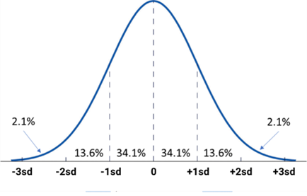
Standard Deviation
Standard deviation (SD) describes the degree of clustering around the average in a normal distribution. For example, we expect 68.2% of all profits and losses to be within one SD of the average; 95.4% within two; 99.6 within three and so on, including any fractional SD values.
For blackjack, the SD varies between 1.14 and 1.17 SD units depending on the table rules, but to keep things simple, let’s use 1.17. This value has been confirmed by simulating millions of hands of blackjack.
So, how can we use the standard deviation to predict profits and losses?
Let’s start with losses. To calculate the maximum loss a blackjack player will experience with a certain probability, we multiply the standard deviation for blackjack by several variables that reflect the total amount of money the player bets then add the effects of the house edge and the player’s basic strategy handicap (his errors). Here’s the formula:
Maximum loss (with 95.4% confidence) =
[ (Standard deviation x 2 SD {for 95.4% confidence}) x
(Square root of the number of hands played) x
(Average bet)
] -
[ ((Average bet) x (Number of hands played) x (House edge)) +
((Average bet) x (Number of hands played) x (Basic strategy handicap))
]
The mathematical reasoning behind this formula is complicated, but here are the highlights:
We multiply the SD by 2 (an approximation) since we want 95.4% confidence (as an example) and need two standard deviations on both the loss and profit side of the normal distribution. (See the normal distribution chart.)
We use the square root of the number of hands played to normalize this value with the SD for blackjack, which has been calculated using the square root of the sum of the variances from the mean.
We need to multiply by the average bet since the standard deviation applies to only one betting unit (i.e., to $1).
We calculate the effect of the house edge by multiplying the house edge by the total amount bet, calculated by multiplying the average bet by the number of hands played.
We calculate the effect of the player’s basic strategy handicap by multiplying the handicap by the total amount bet, calculated by multiplying the average bet by the number of hands played.
To calculate profits, we use the same formula except we subtract the house edge and player’s handicap.